Provides estimation and plotting tools for exposure-response models that use logistic regression for binary responses. It is mostly intended as a convenience package: the core tools are wrappers around glm(), and the plotting tools use ggplot2 and patchwork to build typical plots used in exposure-response modelling.
Models
library(erlr)
library(tibble)

lr_data
#> # A tibble: 300 × 10
#>       id sex      age weight  dose treatment aucss cmaxss   ae1   ae2
#>    <int> <fct>  <int>  <dbl> <dbl> <fct>     <dbl>  <dbl> <dbl> <dbl>
#>  1     1 Male      35     79   200 Drug       673.   97.3     0     1
#>  2     2 Female    22     58   200 Drug      2806.  301.      1     1
#>  3     3 Female    28     58     0 Placebo      0     0       0     0
#>  4     4 Female    18     57   100 Drug      1169.  198.      1     1
#>  5     5 Male      28     77   100 Drug       377.   51.4     0     0
#>  6     6 Female    19     76   200 Drug       327.   25.4     1     0
#>  7     7 Male      30     70     0 Placebo      0     0       0     0
#>  8     8 Female    34     60   100 Drug      1208.  133.      1     1
#>  9     9 Male      21     89     0 Placebo      0     0       0     0
#> 10    10 Female    34     56   200 Drug       254.   31.0     0     0
#> # ℹ 290 more rows

mod <- lr_model(ae1 ~ aucss, lr_data)
mod
#>
#> Call:  stats::glm(formula = formula, family = stats::binomial(link = "logit"),
#>     data = data)
#>
#> Coefficients:
#> (Intercept)        aucss
#>   -1.791383     0.005497
#>
#> Degrees of Freedom: 299 Total (i.e. Null);  298 Residual
#> Null Deviance:       402.1
#> Residual Deviance: 193.4     AIC: 197.4
Plots
lr_data |>
  lr_plot(aucss, ae1) |>
  lr_plot_show_model() |>
  lr_plot_show_quantiles() |>
  lr_plot_show_groups(aucss) |>
  plot()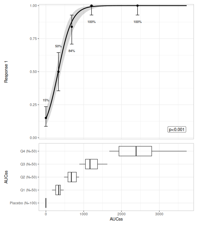
plt <- lr_data |>
   lr_plot(aucss, ae2, stratify_by = sex) |>
   lr_plot_show_model(keep_strata = FALSE) |>
   lr_plot_show_quantiles(bins = 3) |>
   lr_plot_show_datastrip() |>
   lr_plot_show_groups(group_by = c(aucss, treatment), keep_strata = FALSE)

print(plt)
#> <erlr_plot>
#>   plot variables:
#>     - exposure:        aucss
#>     - response:        ae2
#>     - stratification:  sex
#>   plot components:
#>     - model:           ae2 ~ aucss
#>     - quantile:        3 bins
#>     - strip:           jitter both
#>     - group:           .aucss_quantile, treatment
#>   plots built: <none>
#>   output built: no
plot(plt)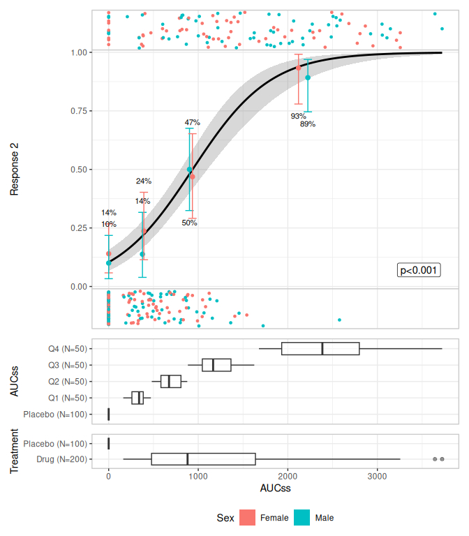
Stepwise covariate modelling
mod1 <- lr_model(ae1 ~ aucss + sex + dose, lr_data)
mod2 <- lr_scm_backward(mod1, candidates = c("sex", "dose"))
#> Using seed = 7932
lr_scm_history(mod2)
#> # A tibble: 4 × 11
#>   iteration attempt step       action term_tested model_tested   model_converged
#>       <int>   <int> <chr>      <chr>  <chr>       <chr>          <lgl>
#> 1         0       0 base model <NA>   <NA>        ae1 ~ aucss +… TRUE
#> 2         1       1 backward   remove ~dose       ae1 ~ aucss +… TRUE
#> 3         1       2 backward   remove ~sex        ae1 ~ aucss +… TRUE
#> 4         2       3 backward   remove ~sex        ae1 ~ aucss    TRUE
#> # ℹ 4 more variables: term_p_value <dbl>, model_aic <dbl>, model_bic <dbl>,
#> #   model_updated <int>
VPC/Simulation
mod <- lr_model(ae1 ~ aucss + sex, lr_data)
sim <- lr_vpc_sim(mod, seed = 1234)
sim
#> # A tibble: 30,000 × 5
#> ae1 aucss sex row_id sim_id
#> <dbl> <dbl> <fct> <int> <int>
#> 1 0.894 673. Male 1 1
#> 2 1.00 2806. Female 2 1
#> 3 0.110 0 Female 3 1
#> 4 0.993 1169. Female 4 1
#> 5 0.588 377. Male 5 1
#> 6 0.468 327. Female 6 1
#> 7 0.129 0 Male 7 1
#> 8 0.994 1208. Female 8 1
#> 9 0.129 0 Male 9 1
#> 10 0.362 254. Female 10 1
#> # ℹ 29,990 more rows
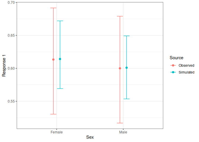
lr_vpc_plot(mod, sim, group_by = aucss)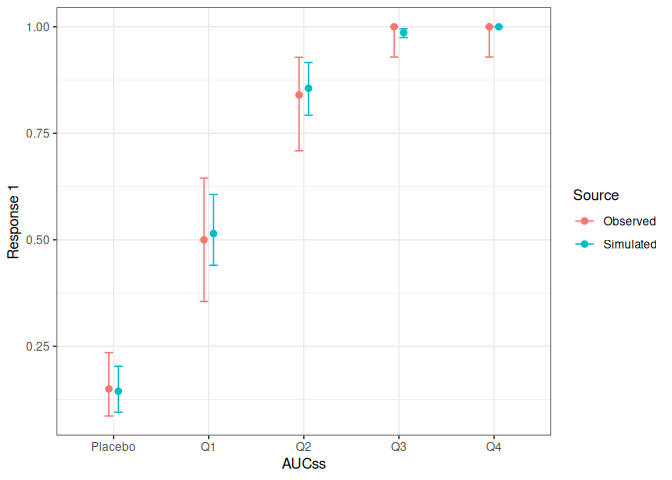
lr_vpc_plot(mod, sim, group_by = sex)