Builds an exposure-response plot for a logistic regression model
Usage
lr_plot(data, exposure, response, stratify_by = NULL)

lr_plot_style(object, labels)

lr_plot_show_model(
  object,
  keep_strata = NULL,
  style = "ribbonline",
  conf_level = 0.95
)

lr_plot_show_quantiles(
  object,
  keep_strata = NULL,
  style = "errorbar",
  bins = 4,
  conf_level = 0.95
)

lr_plot_show_datastrip(
  object,
  keep_strata = NULL,
  style = "jitter",
  panel = "both"
)

lr_plot_show_groups(
  object,
  group_by,
  style = "boxplot",
  bins = NULL,
  keep_strata = NULL
)

lr_plot_build(object)
Arguments
- data
Observed data
- exposure
Exposure variable (one variable, unquoted)
- response
Response variable (one variable, unquoted)
- stratify_by
Stratification variable used for color and fill (one variable, unquoted)
- object
Partially constructed plot (has S3 class
erlr_plot)- labels
Named list of labels
- keep_strata
Logical, indicating whether this component should keep the color stratification
- style
Character string used to specify the partial builder for this component
- conf_level
Confidence level
- bins
Number of exposure bins (not counting placebo)
- panel
Character string: "upper", "lower", or "both" (the default)
- group_by
Grouping variables to define groups for distribution plots (a tidyselection of variables)
Examples
lr_data |>
lr_plot(aucss, ae1) |>
lr_plot_show_model() |>
lr_plot_show_quantiles() |>
lr_plot_show_groups(aucss) |>
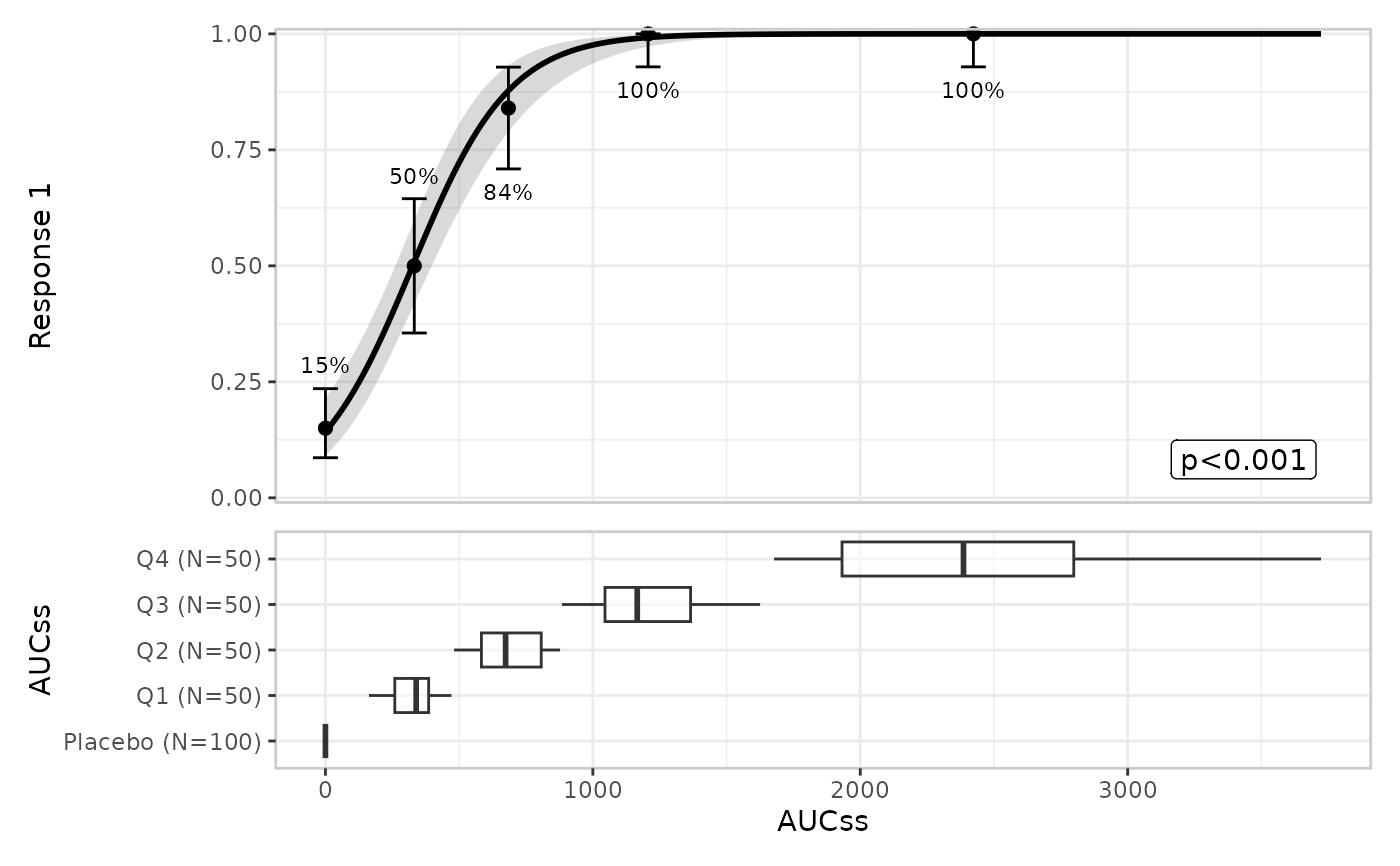
plot()
 plt <- lr_data |>
lr_plot(aucss, ae2, stratify_by = sex) |>
lr_plot_show_model(keep_strata = FALSE) |>
lr_plot_show_quantiles() |>
lr_plot_show_datastrip() |>
lr_plot_show_groups(group_by = c(aucss, treatment), keep_strata = FALSE)
print(plt)
#> <erlr_plot>
#> plot variables:
#> - exposure: aucss
#> - response: ae2
#> - stratification: sex
#> plot components:
#> - model: ae2 ~ aucss
#> - quantile: 4 bins
#> - strip: jitter both
#> - group: .aucss_quantile, treatment
#> plots built: <none>
#> output built: no
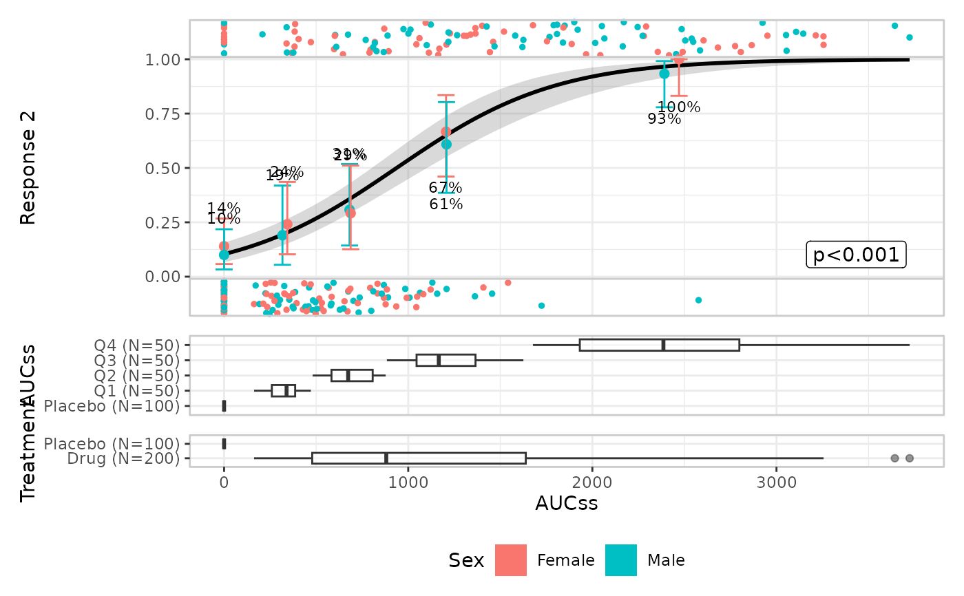
plot(plt)
plt <- lr_data |>
lr_plot(aucss, ae2, stratify_by = sex) |>
lr_plot_show_model(keep_strata = FALSE) |>
lr_plot_show_quantiles() |>
lr_plot_show_datastrip() |>
lr_plot_show_groups(group_by = c(aucss, treatment), keep_strata = FALSE)
print(plt)
#> <erlr_plot>
#> plot variables:
#> - exposure: aucss
#> - response: ae2
#> - stratification: sex
#> plot components:
#> - model: ae2 ~ aucss
#> - quantile: 4 bins
#> - strip: jitter both
#> - group: .aucss_quantile, treatment
#> plots built: <none>
#> output built: no
plot(plt)